
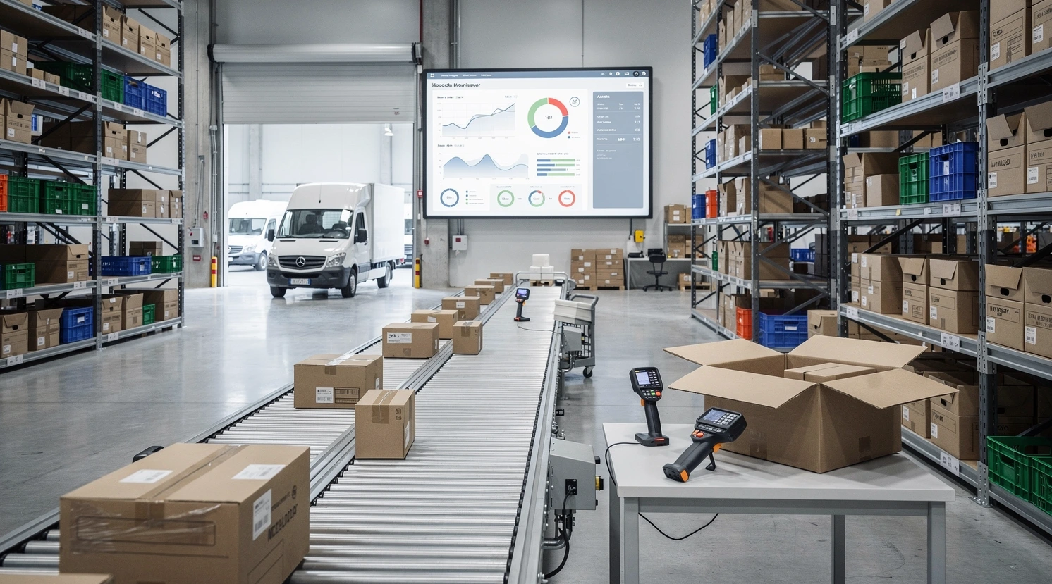
Every retailer who has frozen the floor for an annual physical count knows the sinking feeling on Monday morning: two days of labor burned, and the numbers are already drifting again. Cycle counting replaces that ritual with a rolling discipline that counts a slice of warehousing inventory every day, so accuracy stays high without ever shutting down receiving or picking. Done right, it turns inventory accuracy from an annual gamble into a controllable operating metric you can report on weekly.
This guide is built for operators who actually run the floor: receiving managers, inventory analysts, and store-ops leads who own the stockroom. It covers how to segment SKUs, set count frequencies that survive a busy season, investigate variances without halting the line, and tie the whole program to the inventory accuracy targets your finance team already cares about.
In short
- Cycle counting counts a small subset of SKUs daily on a rotating schedule, so you never freeze operations for a wall-to-wall physical count.
- Segment SKUs with ABC analysis: A items (top 70-80% of value) get counted most often, C items least often, and the cadence follows value and movement, not shelf order.
- The metric that matters is inventory record accuracy (IRA) at the unit level, and best-in-class retail operations hold 97% or higher.
- Variances are signals, not chores: investigate root cause (receiving error, mis-pick, theft, system mapping) before you adjust the on-hand.
- A program pays for itself by cutting stockouts, killing phantom inventory, and removing the annual count’s labor spike.
What is cycle counting, and why does it beat the annual count?
Cycle counting is a method of auditing inventory by counting a defined subset of locations or SKUs on a recurring schedule, rather than counting everything at once. Instead of one disruptive event per year, you count a handful of bins every working day, cycling through the whole catalog over weeks or months depending on how you weight each item.
The annual physical count has two structural problems. First, it produces a single accurate snapshot that decays immediately: by the time the count is reconciled, fresh receipts and picks have already introduced new errors. Second, it forces an operational freeze that costs labor and sales, and the time pressure of a one-day count actually generates miscounts of its own. Cycle counting spreads the effort thin enough that a counter can be careful, and it catches errors within days of them happening, while the cause is still traceable.
The accuracy payoff compounds across the business. Reliable on-hand numbers feed reorder points, prevent overselling on the website, and let you trust automated replenishment. If you want the broader operational context for how accurate stock data underpins shipping and fulfillment economics, our pillar on negotiating shipping rates with UPS and FedEx without losing it shows why clean inventory data is a prerequisite before you ever sit down at a carrier negotiation.
There is also a quieter operational gain. Because cycle counts happen during normal hours, the same staff who pick and put away do the counting, which means they learn the layout cold and start spotting problems (a crushed carton, a mislabeled bin, a slotting error) that a temporary annual-count crew would walk right past. Accuracy improves, and so does the team’s ownership of the stockroom. The annual count, by contrast, is often staffed by people who have never touched the SKUs and have one job: get a number, fast.
The hidden cost of phantom inventory
Phantom inventory is stock the system says you have but the shelf does not. It is the single most expensive symptom of poor warehousing inventory hygiene because it is invisible until a customer orders it. The website accepts the order, the picker walks to an empty bin, and now you are issuing a refund or an apology plus a backorder. Cycle counting surfaces these gaps continuously instead of letting them accumulate until the annual count exposes a year’s worth at once.
The reverse problem, hidden surplus, is just as corrosive even though it never triggers a customer complaint. Stock the system thinks is gone sits in a bin earning nothing, blocking the slot, and tying up working capital. Buyers reorder against an understated on-hand and overstock the SKU, which later gets marked down to clear. Surplus errors do not announce themselves, so only continuous counting catches them. Netting a surplus in one bin against a shortage in another, a common reporting shortcut, hides both at once and is precisely why accuracy must be measured location by location.
Segment your SKUs with ABC analysis before you count anything
The fastest way to waste a cycle-counting program is to count every SKU at the same frequency. A $0.40 fastener does not deserve the same attention as a $400 hero product. ABC analysis ranks items by annual consumption value (unit cost times annual movement) and sorts them into tiers, then you assign count frequency by tier.
The classic Pareto split holds in most retail catalogs: a small fraction of SKUs drives the majority of inventory value. Count the high-value movers often, the long tail rarely, and you concentrate counting labor exactly where errors hurt most.
| Tier | Share of SKUs | Share of value | Typical count frequency | Counts per year |
|---|---|---|---|---|
| A | 10-20% | 70-80% | Monthly | 12 |
| B | 20-30% | 15-25% | Quarterly | 4 |
| C | 50-70% | 5-10% | Twice yearly | 2 |
Two refinements separate a mature program from a textbook one. First, weight by movement velocity, not just value: a moderately priced item that turns 40 times a year touches more hands and accrues more error than a pricey item that sits, so it earns a higher count frequency regardless of its dollar tier. Velocity logic connects directly to how fast stock moves through the building, which we unpack in inventory turnover and why retailers obsess over it. Second, layer in control-group counting for new or problem SKUs: count a small fixed set of items daily for several weeks to expose systemic process errors (a mislabeled bin, a unit-of-measure mismatch) that random sampling would take months to find.
Build the counting calendar
Translate the tiers into a daily quota. If you carry 5,000 SKUs split 15/25/60 across A/B/C, your annual count demand is roughly (750 A items times 12) plus (1,250 B items times 4) plus (3,000 C items times 2), which lands near 20,000 line counts per year. Spread across about 250 working days, that is roughly 80 counts a day, a quota one or two counters can clear in an hour or two without disrupting picking.
Build slack into the calendar from day one. A schedule that assumes 100% completion every day will collapse the first time a counter calls in sick or a truck arrives early, and once you fall behind you tend to stay behind. Plan the quota at roughly 80% of theoretical capacity so a single counter can absorb a normal day’s interruptions and still clear the list. Stagger the start times too: counting before the first wave of orders releases keeps the floor calm and gives you clean, undisturbed bins, which is far easier than chasing accuracy in the middle of a pick storm.
One scheduling decision separates SKU-based from location-based programs. SKU-based counting follows the item wherever it lives, which suits catalogs where one product sits in a single primary location. Location-based counting walks every bin in a zone on a rotation regardless of what is in it, which suits operations with heavy bin-to-bin transfers and forward-pick replenishment, because it catches stock that landed in the wrong slot. Most retail stockrooms run a hybrid: location-based sweeps for the bulk reserve and SKU-frequency counting for the high-value forward-pick face.
Run the count: a repeatable workflow that does not stop the floor
The discipline lives in the procedure. A loose count produces variances you cannot trust, which trains the team to ignore them. Lock the workflow so every count is comparable and auditable.
- Generate the day’s count list from the schedule, sorted by location to create an efficient pick path through the racks.
- Blind count the location: the counter records what is physically there without seeing the system on-hand, which prevents the bias of counting toward the expected number.
- Capture by scan using a handheld or mobile device tied to the WMS, so the location and SKU are confirmed and the count timestamps automatically.
- Compare against system on-hand and flag any location outside tolerance for a recount before any adjustment posts.
- Recount flagged bins by a second person; if the recount confirms the variance, route it to investigation rather than auto-adjusting.
- Investigate root cause, document it, then post the adjustment with a reason code so trends are reportable.
- Feed findings back into the schedule: a bin that misses tolerance gets bumped up in frequency until it stabilizes.
Freeze the location only for the seconds it takes to count, not the whole zone. Modern warehouse management systems let you place a soft hold on a single bin during a count so picks elsewhere continue uninterrupted. That granularity is what lets cycle counting coexist with same-day order flow, including the tight delivery windows covered in our look at the 2026 last-mile delivery outlook for US retailers, where every minute of stockroom downtime ripples into missed cutoffs.
Set tolerance thresholds that mean something
A variance tolerance defines how much discrepancy you accept before triggering investigation. Tolerances should be tighter for high-value A items (often zero units of variance) and looser by percentage for high-count C items, where a single miscount on a 2,000-piece bin of screws is trivial. Define tolerance in both unit and dollar terms so a small percentage swing on an expensive item still trips the flag.
A worked example makes the dual threshold concrete. Suppose an A-tier SKU costs $250 a unit and a C-tier fastener costs $0.30. A flat 2% tolerance would let a $250 item drift by five units (a $1,250 swing) before anyone looked, while flagging a harmless three-piece miss on the fasteners. Set the A item to zero-unit tolerance and the fastener to a 3% or 50-cent band, and the system now investigates the expensive variance and ignores the trivial one. The rule of thumb: tolerance protects dollars first, units second, and you express it as whichever threshold is tighter for that SKU.
Measure what matters: IRA, not raw count totals
The headline metric is inventory record accuracy (IRA), measured as the percentage of locations counted that fall within tolerance. Crucially, measure IRA at the location-SKU level, not by netting overpluses against shortages across the warehouse, which can mask offsetting errors and flatter your numbers.
| Metric | How to calculate | Healthy target | What it tells you |
|---|---|---|---|
| Inventory record accuracy | Locations within tolerance / total counted | 97%+ | Trustworthiness of on-hand data |
| Net dollar variance | Sum of adjustments by value | Trending toward zero | Financial impact and shrink direction |
| Variance frequency by reason code | Count of each root cause | Receiving and mis-pick falling | Where process is breaking |
| Count completion rate | Counts done / counts scheduled | 95%+ | Whether the program is actually running |
Report these weekly to operations and monthly to finance. When IRA holds above 97% for a full quarter, you have earned the right to drop the annual physical count entirely, which most external auditors will accept given a documented cycle-counting program with reason-coded adjustments. That same data discipline is what lets you scale cleanly across channels, a point we develop in the complete guide to selling on global e-commerce marketplaces, where every connected channel inherits whatever inaccuracy lives in your core stock record.
Resist the urge to report a single blended accuracy number. A warehouse-wide 96% can hide a C-tier accuracy of 99% propping up an A-tier accuracy of 88%, which is the dangerous combination: your most valuable, most ordered items are the least accurate. Segment the IRA report by tier so the number that lands in front of finance reflects dollar risk, not piece count. When you do net dollar variance, track the absolute value of adjustments as well, because a net near zero can mask large offsetting errors that signal a process breaking in two directions at once.
Trend matters more than any single reading. A program that posts 95% one week and 99% the next is unstable even if the average looks fine, and the swing usually points to an inconsistent counting procedure rather than real stock movement. Plot IRA as a rolling four-week line, annotate it when you change process (a new scanner, a relocated receiving dock), and you turn the metric into a feedback loop instead of a scorecard. The goal is a high number that barely moves.
Common mistakes that quietly sink a cycle-counting program
Most programs do not fail loudly. They erode as counters cut corners and managers stop reading the variance report. Watch for these patterns:
- Counting with the system on-hand visible. The single most common error. Once a counter sees the expected number, they count toward it, and you are auditing nothing. Always count blind.
- Adjusting first, investigating never. If you auto-post every variance, you erase the evidence trail and lose the ability to fix the process that caused it. The adjustment is the last step, not the first.
- Treating all SKUs equally. Flat-frequency counting wastes labor on the long tail and under-counts the A items where dollar variance concentrates.
- Ignoring receiving as the error source. A large share of inventory variance is born at the dock from miscounts and wrong unit-of-measure entries, not on the pick line. If counts keep missing on freshly received SKUs, fix receiving, not the counters.
- No accountability loop. Counts that nobody reviews train the team that the work does not matter. Someone must own the weekly IRA number.
- Letting the schedule slip during peak. Suspending counts in Q4 is exactly backward: that is when movement and error are highest. Reduce the daily quota if you must, but keep the cadence alive.
Frequently asked questions
How often should I cycle count?
Frequency follows value and velocity, not a single calendar rule. Under a standard ABC scheme, high-value A items are counted monthly, mid-tier B items quarterly, and low-value C items twice a year. Fast-moving items get bumped up a tier regardless of cost because movement drives error. The practical anchor is your daily quota: divide total annual line-counts across your working days, and a single counter clearing 60 to 100 counts a day keeps a mid-size catalog fully covered without disruption.
What inventory accuracy percentage is realistic for retail?
Best-in-class retail operations sustain inventory record accuracy of 97% or higher at the location-SKU level. Below roughly 95%, automated replenishment and online order promising become unreliable and you will see stockouts and oversells. The target is not 100%: chasing perfect accuracy on low-value C items burns labor with no payback. Set tier-specific tolerances so effort lands where dollar risk is, and measure accuracy by counting matches, not by netting surpluses against shortages, which hides offsetting errors.
Can cycle counting replace the annual physical count?
Yes, in most cases. A documented cycle-counting program that holds IRA above 97%, posts reason-coded adjustments, and maintains a complete count history is generally accepted by external auditors as a substitute for a wall-to-wall physical inventory. The substitution removes the annual labor spike and the operational freeze. The condition is rigor: blind counts, second-person recounts on variances, and an auditable trail. Without that discipline, auditors will still demand the full physical count.
What causes most inventory variances?
The biggest sources are receiving errors (miscounts and wrong unit-of-measure entries at the dock), mis-picks during fulfillment, misplaced stock in the wrong bin, and theft or shrink. System mapping issues, such as a SKU pointing to the wrong location, also generate phantom variances. The value of reason codes is that they tell you which cause dominates. If receiving drives your variances, no amount of recounting fixes it; you correct the inbound process instead.
Do I need a WMS to cycle count?
You can start with a spreadsheet and a clipboard, but a warehouse management system multiplies the program’s value. A WMS generates location-sorted count lists, supports blind counts by hiding on-hands, captures scans with timestamps, applies single-bin holds so picking continues during a count, and stores reason-coded variance history for reporting. For any operation past a few hundred SKUs, the manual approach gets fragile fast. Treat the WMS as the system of record and never let counters edit on-hands directly outside the count workflow.
How do I count blind without slowing the team?
Blind counting means the counter records the physical quantity without seeing the system’s expected number, then the system compares afterward. It costs almost nothing in time: the counter still walks one path and scans each bin once. The comparison and flagging happen automatically. The only added step is the second-person recount on flagged locations, which applies to a small fraction of counts when accuracy is healthy. The bias removal is worth far more than the marginal seconds, because a non-blind count audits nothing.
What’s next
Start by running an ABC analysis on last year’s movement data and standing up a daily count quota for just your A items, then expand the cadence outward as the workflow stabilizes and your IRA climbs past 97%. Once your on-hand numbers are trustworthy, the rest of the logistics stack gets easier to optimize, from replenishment timing to the carrier conversations laid out in negotiating shipping rates with UPS and FedEx without losing it. For the standards that auditors and finance teams lean on when they evaluate inventory controls, the ASCM/APICS body of knowledge is the reference operators cite most.