
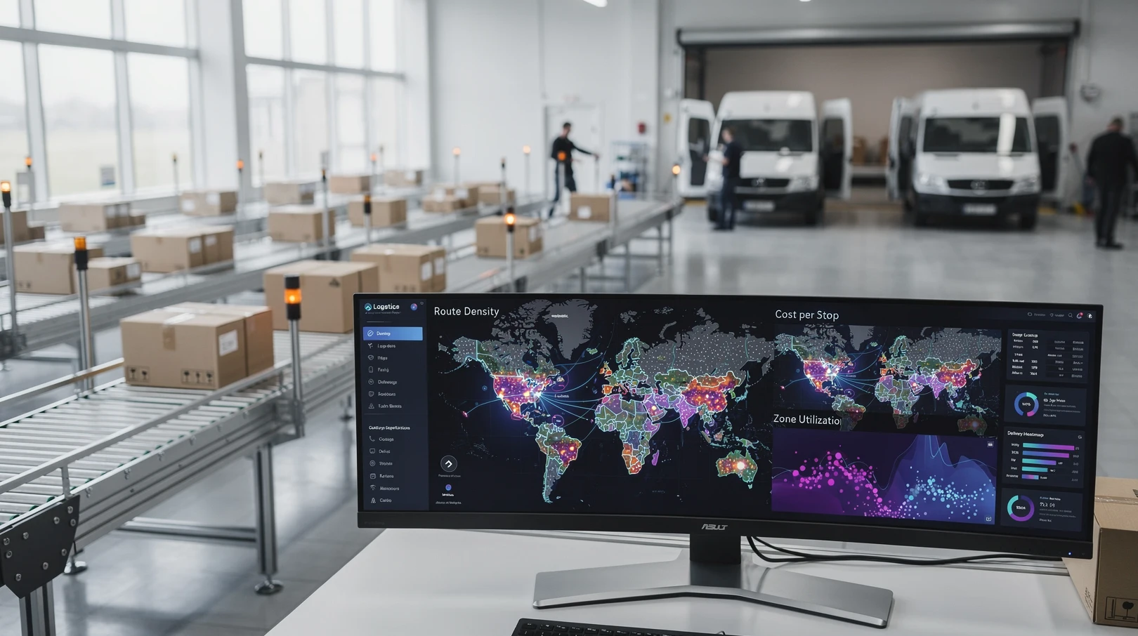
Two retailers can pay a courier the exact same per-stop contract rate and still see last mile delivery costs that differ by 40 percent. The variable that separates them is not the carrier, the box size, or even the fuel surcharge. It is delivery density: how many drop-offs a driver completes per hour inside a defined service area. Density is the quiet multiplier behind every shipping invoice, and most merchants never measure it because it never appears as a line item.
This guide treats density as a number you can manage, not a market condition you accept. We will define it precisely, show how it bends your cost per parcel, and walk through the levers (zone design, time windows, pickup points, and order batching) that move the needle. The same math that lets Amazon run a route for under two dollars a stop is available to a regional brand shipping 800 orders a week, provided you read your own map correctly.
The stakes are larger than a few cents per box. For most omnichannel retailers, the last mile is the single most expensive leg of the supply chain, often consuming half of total fulfillment cost while covering the shortest distance. A package can travel 2,000 miles across the country for less than it costs to move the final two miles to a customer’s door, because the line-haul leg is dense and automated while the last mile is fragmented and manual. Density is the metric that decides whether that final leg is a margin sink or a competitive moat.
In short
- Delivery density is stops per route-hour inside a service area; it is the strongest single driver of last-mile cost, ahead of distance or parcel weight.
- Doubling drops per square mile typically cuts cost per parcel by 25 to 35 percent because the fixed costs of a route (driver wage, vehicle, depot return) spread across more packages.
- Carriers already price density through zone surcharges, residential fees, and extended-area charges; your invoice reflects your map whether you optimize it or not.
- Merchants raise density with pickup points, scheduled delivery windows, order-batching incentives, and tighter geographic targeting, not by switching couriers.
- Track cost per successful delivery by ZIP cluster, not blended shipping spend, or you will subsidize your sparsest routes forever.
What delivery density actually measures
Density is the count of successful deliveries a driver completes per hour of active routing inside a bounded zone. A dense urban route might post 18 to 25 stops per hour; a rural route covering the same calendar hour may post 4 to 6. The driver costs the same in both cases, so the sparse route spends two to four times more labor per parcel before a single package leaves the van. The same logic governs the depot behind the route, and if you are still sizing your fulfillment footprint, our walkthrough of warehousing basics for growing retail brands covers how depot placement feeds directly into route economics.
The reason density dominates is structural. A delivery route carries a stack of fixed costs: the driver’s shift wage, the vehicle lease, fuel for the trunk run from depot to neighborhood, and the return leg. Those costs exist whether the van drops 40 parcels or 140. Density is simply the denominator that those fixed costs are divided by. Distance and parcel weight do move the needle, but they are second-order effects: a route’s labor clock keeps running regardless of how much each box weighs, which is why a heavier, denser route still beats a light, scattered one on cost per parcel.
Carriers understand this better than most shippers, which is exactly why your rate card is full of geographic modifiers. When you later sit down to negotiate shipping rates with UPS and FedEx, you will find that zone-based pricing, delivery area surcharges, and residential adders are all density proxies dressed up as fees. The carrier is charging you for the shape of your customer map.
It helps to separate density from two metrics it gets confused with. Drop size is the number of parcels delivered at a single address, which matters but is usually small for direct-to-consumer retail. Stop density is the number of distinct addresses per route mile or per route-hour, and this is the figure that governs last-mile economics for most merchants. A van that drives three miles between two homes burns the same labor and fuel as one making twelve stops over those three miles, but the second route serves six times the orders. When this guide says density, it means stop density measured against route-hours, because time, not distance, is what you are buying when you pay a driver.
There is also a temporal dimension that pure geography misses. Two routes can cover identical neighborhoods yet post very different stops-per-hour if one runs at rush hour and the other mid-morning. Traffic, parking difficulty, building access, and the time spent walking from curb to door all eat into the hour. Dense urban cores with high-rises can paradoxically slow a driver despite short distances, because elevator waits and lobby check-ins stretch the dwell time at each stop. Real density management means watching the clock, not just the map.
How density translates into cost per parcel
Answer first: every additional stop per route-hour lowers your cost per parcel along a predictable curve, and the steepest savings come at the low end. Going from 6 to 12 stops per hour saves far more per parcel than going from 24 to 30, because you are halving the fixed-cost allocation rather than trimming it.
The table below models a single eight-hour route with a fully loaded daily cost of 360 dollars (driver, vehicle, fuel, depot overhead). Watch how the cost per delivery collapses as density climbs while the route cost stays flat.
| Stops per route-hour | Deliveries per 8-hour day | Daily route cost | Cost per delivery |
|---|---|---|---|
| 6 (sparse rural) | 48 | $360 | $7.50 |
| 10 (suburban) | 80 | $360 | $4.50 |
| 15 (dense suburban) | 120 | $360 | $3.00 |
| 20 (urban) | 160 | $360 | $2.25 |
| 25 (high-rise urban) | 200 | $360 | $1.80 |
The curve is hyperbolic, not linear. A retailer stuck at 6 stops per hour who reaches 10 cuts cost per delivery by 40 percent. That is the same magnitude of saving most merchants chase through carrier negotiation, except density is a lever you control through your own fulfillment design rather than a concession you beg for. Notice also that the savings flatten at the top: moving from 20 to 25 stops trims only 45 cents per delivery, so the highest-density urban operations have already harvested most of the available efficiency and should pour their energy into their thin zones instead.
The model above uses a flat 360 dollar route cost for clarity, but in practice the cost itself is not perfectly fixed. Above a certain stop count, drivers may need more hours, the van may need a second loading trip, or you may add a route entirely. The useful planning rule is that costs are fixed within a route’s capacity band and step up only when you cross into a new van or shift. Your job is to fill each route’s capacity before you spin up the next one, because a half-empty second route is the most expensive parcel you will ever deliver.
Translate this into annual money and the priority becomes obvious. A merchant shipping 200,000 parcels a year who moves blended cost from 4.50 to 3.00 dollars per delivery saves 300,000 dollars, more than most carrier renegotiations return, and the savings recur every year without an annual round of haggling. Density is the gift that keeps giving because it is structural, not contractual.
Density also explains why same-day service punishes thin routes so severely: compressing delivery windows shrinks the geographic pool a single van can cover, which mechanically lowers stops per hour. Our breakdown of same-day delivery economics for retailers shows where that tradeoff pays off and where it quietly burns margin.
The levers that raise density
Answer first: you raise density by concentrating drops in space and time. Five levers do most of the work, and they compound when stacked. Here they are in the order most retailers should attack them.
- Pickup points and lockers. Routing 30 percent of orders to a single locker bank converts dozens of scattered home stops into one high-volume drop, instantly lifting effective density and cutting failed-delivery reattempts to near zero.
- Scheduled delivery windows. Offering customers a “Tuesday or Thursday” choice lets you batch a neighborhood into one route day instead of dribbling parcels across five, doubling or tripling local stop counts.
- Geographic order targeting. Free-shipping thresholds and regional promotions steer demand toward ZIP clusters where you already run dense routes, deepening your strongest zones rather than spreading thin.
- Order batching and consolidation. Holding multi-item orders for a single combined dispatch, and merging same-household orders, raises parcels per stop without changing the route at all.
- Depot and micro-fulfillment placement. Positioning inventory closer to demand shortens the unproductive trunk run, returning more of the shift to productive stops.
None of these requires a new carrier contract. They are operational and merchandising decisions that reshape the map your existing courier already prices against. The macro context matters too: shifting consumer expectations around speed and free shipping change which levers are viable, and our explainer on how retail news shapes the global e-commerce industry tracks the demand-side forces that set those expectations.
Sequencing matters as much as the levers themselves. Pickup points and scheduled windows are demand-shaping moves that change customer behavior, so they take weeks to ramp and depend on adoption rates. Order batching and consolidation are operational moves you can switch on immediately inside your warehouse with no customer-facing change at all. Start with the operational levers for fast wins, then layer in the demand-shaping ones to lock in the gains. A merchant who reverses that order spends months redesigning checkout flows while leaving easy batching savings on the table.
A worked example: shrinking a thin zone
Answer first: the fastest path to lower blended cost is to attack your worst cluster, not to nudge your best. Consider a regional apparel brand shipping 1,000 parcels a week, with 70 percent concentrated in two metro clusters running at 14 stops per hour and 30 percent scattered across rural ZIP codes running at 5 stops per hour. The rural tail is only 300 parcels but, at roughly 9 dollars per delivery, it consumes nearly as much delivery budget as the 700 profitable urban parcels combined.
The brand applies three moves to the rural tail. It places parcels at two regional locker banks that 40 percent of rural customers agree to use in exchange for a one dollar discount, converting scattered home stops into two consolidated drops. It shifts the remaining rural deliveries to a single weekly route day so the van batches the whole tail into one trip instead of three. And it raises the free-shipping threshold for rural ZIP codes from 50 to 75 dollars, nudging order values up so each parcel carries more margin to absorb its higher cost. Within a quarter the rural cluster’s effective cost per delivery falls from 9 dollars toward 6, and the blended figure across the whole book drops by roughly 18 percent. No carrier negotiation took place.
The lesson generalizes: your blended cost is an average dragged down by a minority of bad routes. Surgically improving the worst 20 to 30 percent of your geography moves the average far more than squeezing the routes that already run well.
Reading density off your own map
Before you can manage density you have to measure it, and blended shipping spend hides everything. The fix is to segment cost by ZIP cluster and compute cost per successful delivery for each. A handful of sparse clusters almost always drag the average, and you may be charging every customer a flat shipping fee that subsidizes the most expensive 10 percent of your geography.
Map your last 90 days of deliveries onto ZIP clusters, then sort by stops-per-route-hour. The pattern is usually stark: a few dense clusters carry profitable margins while a long tail of thin clusters loses money on every parcel. Once you see it, the decisions write themselves. You can raise shipping fees in thin zones, push those customers toward pickup points, or set free-shipping thresholds high enough to cover the route cost. Authoritative carrier cost research from the U.S. Bureau of Labor Statistics on transportation labor confirms that driver wages, not fuel or vehicles, are the dominant and least compressible last-mile cost, which is precisely why spreading them across more stops matters so much.
Build a simple density scorecard with four columns per cluster: parcels per week, stops per route-hour, cost per successful delivery, and first-attempt success rate. That last column is the one most retailers forget, and it is where money silently leaks. A cluster that looks dense on paper but posts a 12 percent failed-delivery rate is effectively far sparser than its raw numbers suggest, because every reattempt is a second stop with no second order. Pairing density with first-attempt success gives you the true cost picture.
Refresh the scorecard quarterly, because your map is not static. Marketing campaigns, new store openings, and seasonal demand all shift where parcels land. A cluster that was thin in spring may densify after a regional promotion, flipping it from a candidate for surcharges to a candidate for faster service. Treat density as a living operating metric reviewed alongside revenue, not a one-time logistics study that gathers dust.
Finally, connect the scorecard back to merchandising. The clusters where you already run dense, cheap routes are exactly where aggressive free-shipping offers and fast-delivery promises pay off, because the marginal parcel there costs almost nothing to move. Targeting promotions at your dense zones deepens your cost advantage, while blanket nationwide free shipping quietly funds your most expensive routes. Density data turns shipping from a flat cost center into a precision merchandising tool.
Common mistakes
The first mistake is treating shipping as a single blended number. A flat 6 dollar cost per parcel across your whole footprint conceals 2 dollar urban routes and 12 dollar rural ones, and you cannot fix what you average away.
The second is chasing carrier discounts while ignoring density. A 5 percent negotiated rate cut is real money, but moving a thin route from 6 to 12 stops per hour delivers a 40 percent reduction. Merchants routinely spend months on the smaller lever and never touch the larger one.
The third is over-promising speed in low-density zones. Offering same-day or next-day windows to a rural customer base forces tiny, expensive routes that no shipping fee fully recovers. Match your service promise to your map, not to a competitor’s urban marketing.
The fourth is ignoring failed deliveries. A reattempt doubles the effective cost of that stop and corrupts your density math; pickup points and confirmed windows are the cheapest insurance against this hidden tax.
FAQ
What is a good delivery density to aim for?
There is no universal target because density is bounded by your customer geography, but the useful benchmark is internal improvement. If your suburban routes run at 8 to 10 stops per route-hour, pushing toward 14 to 16 through batching and windows is realistic and cuts cost per parcel by roughly a third. Urban operations can reach 20 to 25. Rural zones may cap near 6 regardless of effort, which is your signal to shift those customers toward pickup points or higher shipping fees rather than fighting the map.
Does delivery density matter if I use a national carrier instead of my own fleet?
Yes, and arguably more, because the carrier prices density into your rate card through zone charges, delivery area surcharges, and residential adders. You do not see the stops-per-hour figure, but you pay for it. Concentrating your orders in dense ZIP clusters lowers the surcharges you trigger and strengthens your hand when you negotiate. The lever is the same whether you run vans or hand everything to UPS: a tighter, denser customer map costs less to serve.
How do pickup points improve density so dramatically?
A pickup point converts many individual home stops into one consolidated drop. Instead of a driver making 15 separate residential deliveries across a neighborhood, the van makes one stop at a locker bank and unloads 15 parcels in minutes. That single change can lift effective stops-per-hour sharply while eliminating the failed-delivery reattempts that plague residential routes. The customer absorbs the final few hundred meters, which is the most expensive segment of the entire journey.
Can scheduled delivery windows actually raise density?
They are one of the most effective levers available. When customers self-select a day, you can batch an entire neighborhood into one route instead of sending vans into the same area on multiple days for one or two parcels each. The result is more drops per route and fewer wasted miles. The tradeoff is a slightly slower promise to the customer, so windows work best for non-urgent categories where buyers value reliability over raw speed.
How do I measure delivery density without a transportation management system?
A spreadsheet is enough to start. Export your last 90 days of orders with delivery ZIP codes, group them into clusters, and divide deliveries by the route-hours your carrier or fleet logged in each cluster. Even a rough estimate exposes the thin zones dragging your blended cost. The goal at this stage is not precision but ranking: identify which clusters are profitable and which are subsidized, then aim your operational changes at the worst offenders first.
Does higher density ever hurt service quality?
It can if you push it past the point where drivers have time to complete each stop properly. Cramming too many drops into a route creates rushed handoffs, missed delivery instructions, and rising complaint rates. The sweet spot raises density while keeping enough buffer for the average stop to be done correctly the first time. Failed or disputed deliveries destroy the cost savings density was supposed to create, so track first-attempt success alongside stops-per-hour.
What’s next
Pull your last quarter of deliveries into ZIP clusters this week and compute cost per successful delivery for each, then rank them. Once you can see which zones subsidize which, the operational moves (pickup points for thin clusters, scheduled windows for the rest) become obvious. From there, revisit your carrier terms with density data in hand, because the same map that drives your internal route cost is the lever you bring to the table when you negotiate shipping rates with UPS and FedEx for a sharper contract.