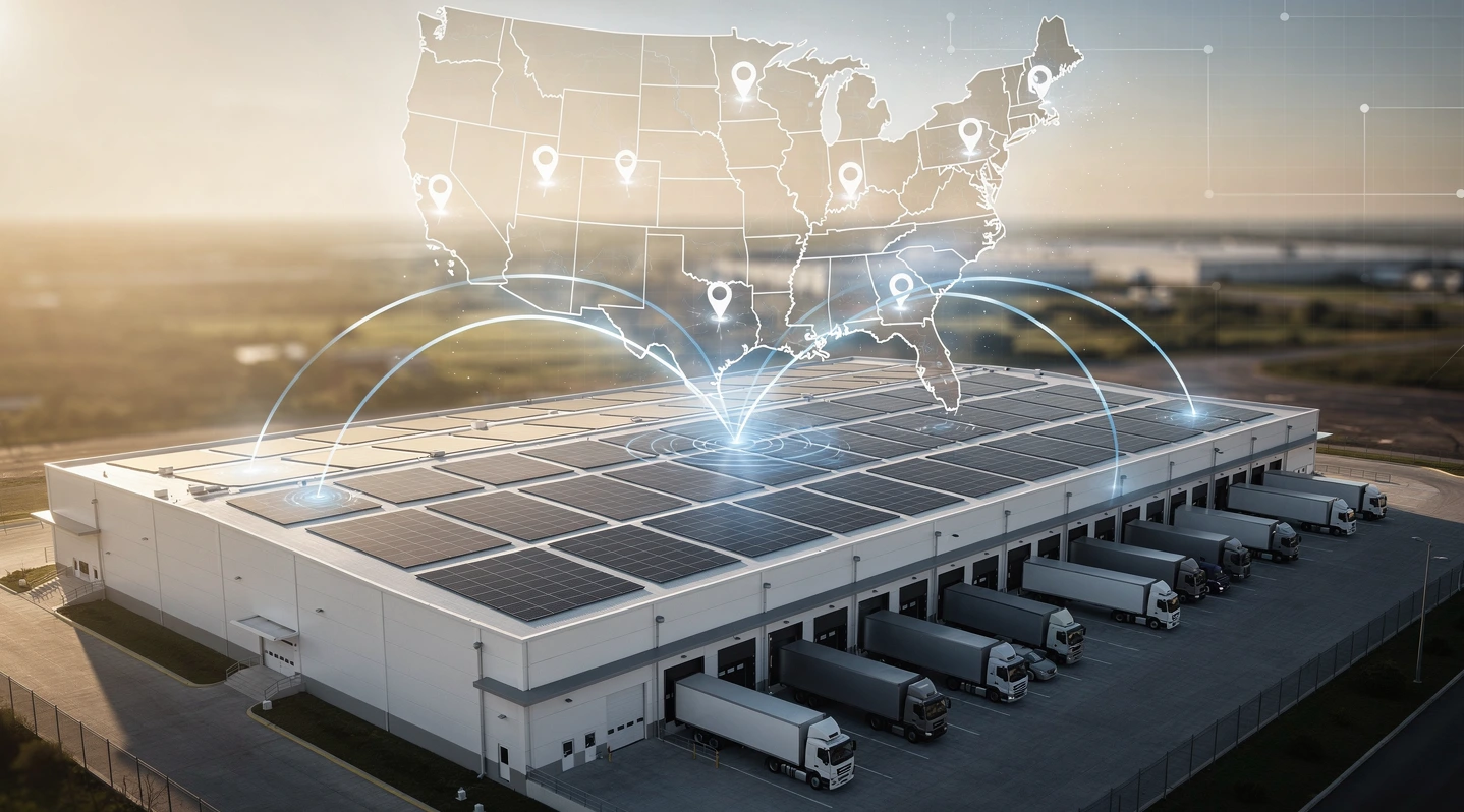
Fulfillment center locations math is the spreadsheet behind every retail brand that ships on time without bleeding margin. It is the work that decides whether a customer in Phoenix gets a package in one day or four, whether your shipping subsidy line stays under 8% of revenue, and whether a new product launch survives Cyber Week. Most US retailers treat it as a one-off real estate decision. The brands that win treat it as an ongoing optimization problem with clear inputs, clear constraints, and an answer that changes every twelve to eighteen months.
In short
- Network design is a math problem first, a real estate problem second. Start with your customer density map, weighted by order frequency, before you tour a single warehouse.
- Two well-placed nodes can cover roughly 80% of the US population in two days via ground shipping, while three to four nodes push next-day coverage past 60%.
- The right number of fulfillment centers is the one where the next center adds more transportation savings and customer retention than it adds in fixed cost.
- Most networks fail on tail SKUs, not on hero SKUs. Splitting inventory across nodes raises holding cost and split-shipment rates if your forecasting cannot keep up.
- Greenfield models, p-median, and weighted centroid analysis are the three methods worth knowing, and they answer different questions.
This piece is part of our cluster on shipping and fulfillment, anchored by the pillar guide to modern retail logistics from warehouse to doorstep. If you are still mapping the basics, start there and come back.
Why fulfillment center math matters more in 2026
US shoppers have internalized the two-day default. US Census e-commerce data shows online sales pushing past 16% of total retail in 2026, and the buyers driving that growth do not split hairs between Amazon, Walmart, and your direct-to-consumer site. They click, they wait, and if your promise slips past three days twice in a row, they remember.
The math behind hitting that promise is not glamorous. It is a function of where your customers live, how fast you can hand a package to a carrier, and how much you are willing to spend to compress the last mile. The smaller your brand, the more those three variables matter, because you do not have the freight volume to negotiate the carrier rates that protect bigger retailers from network design mistakes.
There is also a margin story. Outbound shipping is now the single largest variable cost for many mid-size US e-commerce brands after cost of goods. A poorly placed network can quietly add 90 to 180 basis points to that line, which is often the difference between a profitable channel and one that survives on growth-stage financing. Before going deeper, brands that are still figuring out the fundamentals should review our piece on shipping and fulfillment basics for new retail brands, which covers the vocabulary this article assumes.
Key terms behind network design
Fulfillment network design borrows vocabulary from operations research, supply chain, and real estate. The terms get conflated in vendor pitches and that is where bad decisions start.
A fulfillment center (FC) is a warehouse optimized to pick, pack, and ship individual orders to consumers. It is not the same as a distribution center (DC), which moves pallets and cases to retail stores or wholesale buyers. Many brands run hybrid facilities, but the unit economics differ. A pick line designed for parcels rarely runs efficient pallet flow, and vice versa.
A node is any stocking point in your network, including FCs, third party warehouses, and forward stocking locations. A spoke is the lane between a node and a delivery zone. Zone skipping is the practice of trucking parcels from your FC to a carrier injection point closer to the customer, which can cut a ground transit day for a fraction of expedited cost.
A zone, in the US carrier sense, is the distance band between origin and destination ZIP code. UPS, FedEx, and USPS all use a similar zone 1 to zone 8 framework. Zone 2 packages cost roughly half what zone 8 packages cost on the same service level. The whole point of multi-node networks is to push the average zone down toward 3.
Service level is the percentage of orders that hit a promised transit time. Targeting 95% two-day ground in the contiguous US is the working benchmark for direct-to-consumer brands in 2026. Split shipment rate is the percentage of orders where items ship from more than one node. Above 12% it usually means your network is fragmented faster than your inventory math can handle.
How fulfillment location math actually works
The honest answer is that there is no single formula, but there is a sequence of analyses that converges on a defensible answer. The work is iterative, and the inputs need to be refreshed at least annually as your demand mix shifts.
Step one is the customer density heatmap. Pull a year of order data, geocode the destinations to ZIP code, and weight each ZIP by the number of orders and by margin contribution. Plot it. For most US brands the map shows a familiar story: heavy concentration in California, Texas, the Northeast corridor, Florida, and the Chicago-to-Detroit belt. That picture is your input, not your output.
Step two is the weighted centroid calculation. Treat each ZIP as a point with a mass equal to its annual orders. Compute the geographic center. For a typical US consumer brand the answer lands somewhere in Missouri, Kentucky, or Indiana. That centroid is the theoretical best single-node location, ignoring real estate cost, labor availability, and tax. It is also the reason Memphis, Louisville, Indianapolis, and Columbus dominate single-node US fulfillment maps.
Step three is the p-median problem, an operations research staple. Given p potential nodes to open, choose the subset that minimizes total weighted distance from customers to their nearest node. This is the math that decides whether two nodes, three nodes, or five nodes is the right answer. Modern solvers handle 50,000 candidate ZIPs and 200 candidate sites in seconds, so the constraint is data quality, not compute.
Step four is the greenfield model. Take the p-median output, layer in real estate cost per square foot, labor wage data from the Bureau of Labor Statistics, state corporate tax, sales tax nexus implications, and inbound freight cost from your suppliers. Re-rank. The greenfield model is what converts an academic answer into a board-ready proposal.
Step five is sensitivity analysis. Vary demand growth by plus or minus 25%, vary fuel cost by plus or minus 30%, vary the carrier rate card by current published increases. Networks that look optimal at one snapshot but fall apart with mild shocks are the ones that lose money in year two.
A worked two-node example
Imagine a US apparel brand shipping 600,000 parcels a year. Customer density skews 38% West, 24% Northeast, 18% Southeast, 12% Midwest, 8% Mountain and other. A single node in Indianapolis covers the country at an average zone of 4.3 with two-day ground reaching about 48% of orders. The shipping bill runs roughly $5.4 million.
Add a second node in Reno or the Inland Empire. Average zone drops to 3.1, two-day ground coverage jumps to 82%, and the shipping bill falls to roughly $4.1 million. Fixed cost for the second node, including lease, equipment, and a 60-person team, adds about $2.6 million. Holding cost on duplicated inventory adds another $400,000. The net is a swing from $5.4 million all-in to $7.1 million all-in. The second node loses money on logistics alone.
The case only works if the faster delivery promise lifts conversion or repeat purchase by enough to cover the gap. For most apparel brands, that lift is real but smaller than vendors claim. For consumables and beauty, it is usually larger. The math forces an honest conversation about which category you are actually in.
The metrics that actually decide the answer
A network design exercise lives or dies on three KPIs. The first is landed cost per outbound parcel, defined as outbound freight plus FC variable labor plus pro-rated fixed cost, divided by parcels shipped. Tracking it weekly catches drift before it becomes a quarterly surprise.
The second is the order-weighted average zone. This single number explains roughly 70% of the variance in your shipping bill across nodes. If average zone is creeping up after a new launch, it usually means your demand mix has shifted faster than your inventory placement.
The third is perfect order rate: the share of orders that ship on time, complete, undamaged, and accurately. A network that hits 99% perfect order rate is rare, expensive, and almost always over-engineered. A network below 96% is leaking customers in ways that show up in repeat rate, not in any single complaint metric. The sweet spot for most US direct-to-consumer brands lands between 97% and 98.5%.
Common mistakes that wreck a fulfillment network
The patterns repeat across categories, and almost every one shows up in network design decks that were sold as data-driven.
- Designing around historical demand instead of forward demand. If your growth is shifting from coastal cities to secondary metros, a network optimized for last year’s heatmap will be wrong by year two.
- Ignoring inbound freight. A warehouse 200 miles from your supplier’s port of entry can wipe out outbound savings if your inbound volume is heavy and your SKU count is high.
- Splitting inventory before forecasting can support it. Two nodes with bad forecasts produce split shipments, stockouts, and angry customers. One node with good forecasts ships clean every time.
- Choosing labor markets that look cheap on paper. A market with a low base wage but high turnover and thin available workforce ends up more expensive once you include training, overtime, and peak-season agency premiums.
- Treating peak as a footnote. Networks sized for average volume melt during November and December. Peak capacity, not average capacity, is what defines whether the math is honest.
- Underweighting returns. Returns processing can absorb 25% to 40% of a center’s labor hours in apparel and footwear. A network that ignores reverse logistics design is a network that drowns in January.
- Buying real estate before pricing the labor. The cheapest lease in the wrong county is the most expensive operating decision you will make.
- Locking into long leases with no flex space. Five-year leases with no expansion option leave brands paying for storage they cannot use or scrambling for temporary space during peak.
Real US retail examples worth studying
The publicly visible US networks tell a clear story about what experienced operators settle on.
Amazon’s US fulfillment footprint runs more than 110 sortable and non-sortable FCs, paired with hundreds of delivery stations. The density is not driven by inventory math alone; it is driven by the same-day and next-day promise. Most brands cannot afford that geometry and should not try to copy it.
Walmart’s network leans on a different logic. Stores act as nodes for ship-from-store and pickup, which lets the chain reach the country in two days without dedicated e-commerce real estate in every metro. If you have a retail footprint already, the math changes meaningfully.
Chewy operates roughly a dozen fulfillment centers spread across the country with a clear East, Midwest, and West triangle. The clustering reflects bulky, low-margin freight where zone optimization is the largest single cost lever. Beauty and supplements players like Glossier, Olipop, and Athletic Brewing typically run two or three nodes with a 3PL partner, focusing on two-day coverage rather than next-day.
Marketplace-first brands hit a different shape. A US merchant selling on Temu, or running a meaningful Amazon FBA business, often delegates the network math to the marketplace. That works for one channel but creates a fragmentation problem when you eventually open a direct site and discover your owned inventory is in the wrong place to serve your owned customers.
Patagonia gives one of the cleanest case studies in the category. The brand runs a Reno, Nevada anchor node with a smaller East Coast facility, which gives it sub-three-day coverage on roughly 90% of orders while keeping inventory complexity manageable. Reno also sits within a day’s truck reach of the Port of Oakland and the Port of Los Angeles, which compresses inbound freight cost for an import-heavy product line. That is the textbook example of network math that respects both directions of the supply chain, not just outbound.
On the smaller end, brands like Pattern Brands and Caraway typically lean on a single 3PL partner running two to three nodes on their behalf. The unit economics work because they pay variable cost per parcel rather than fixed cost per node, which protects them during launch volatility. The trade-off is that 3PL pick-and-pack rates per unit are usually 10% to 20% higher than what an in-house team can hit at scale, so a partner-based network has a natural ceiling at which insourcing starts to pay back.
What the data says about coverage curves
If you plot two-day ground coverage against number of nodes for a typical US brand, the curve is steeply concave. The first node gets you to about 50% coverage. The second node almost doubles that to 80% to 85%. The third node adds another 7 to 10 percentage points. The fourth and fifth nodes barely move the headline coverage number, but they collapse the average zone for high-value coastal customers, which can matter more than the raw coverage figure if your repeat customers cluster on the coasts. That diminishing return is why most US brands settle at two or three nodes for a long time before adding a fourth.
Tools, partners and 3PLs worth knowing
The toolchain divides into modeling software, real estate intelligence, and operational partners.
On the modeling side, LLamasoft (now part of Coupa) and Optilogic Cosmic Frog dominate enterprise network design. For brands at 200,000 to 5 million annual parcels, custom analytics on top of Google OR-Tools or Gurobi are increasingly common and far cheaper than enterprise licenses. The output should always be reproducible in a spreadsheet, even when the solver runs in Python.
On the real estate side, CBRE, JLL, and Colliers publish quarterly industrial market reports with submarket-level rent, vacancy, and labor data. Treat them as the baseline. A broker who cannot articulate the labor depth of a submarket as well as the lease rate is the wrong broker.
On the operations side, the choice is usually between in-house operations and a 3PL. ShipBob, Saddle Creek, Quiet Logistics, Rakuten Super Logistics, and Radial are common names for direct-to-consumer brands. The trade-offs are large enough that we treat them in their own piece on in-house versus 3PL fulfillment and when to make the switch.
The table below compares the common shapes a US brand can run, with realistic ranges based on what operators actually see in 2026.
| Network shape | Typical use case | Avg zone | 2-day ground coverage | All-in fixed cost |
|---|---|---|---|---|
| 1 node, Midwest | Brands under 200K parcels/year | 4.2 to 4.5 | 45% to 55% | $1.5M to $3M/yr |
| 2 nodes, East + West | 200K to 1.5M parcels/year | 3.0 to 3.3 | 80% to 88% | $3.5M to $6M/yr |
| 3 nodes, East + Central + West | 1M to 5M parcels/year | 2.6 to 2.9 | 90% to 95% | $5M to $9M/yr |
| 4+ nodes, regional | 5M+ parcels, next-day expectations | 2.2 to 2.6 | 95%+ with next-day in 50% | $8M to $20M+/yr |
The table is a starting point, not a recommendation. The right answer for any specific brand still depends on demand mix, SKU count, return rate, and the carrier rate card you can actually negotiate. For the broader operating context across procurement, warehousing, and last mile, the retail logistics pillar guide stitches the pieces together.
How to phase a network expansion without breaking the business
Most network changes fail because the operating team underestimates the transition cost. A clean expansion follows a predictable sequence and you skip steps at your peril.
Pick the next node based on data, not on a real estate deal that landed in your inbox. Confirm the labor depth within a 30-mile radius using state workforce data, not the broker’s flyer. Pre-commit a launch SKU subset, usually 40% to 60% of total SKU count, focused on velocity items that benefit most from zone reduction. Run a four to eight week parallel period where both nodes ship the same SKUs to overlap zones, so you can measure actual carrier performance and labor productivity before flipping the full traffic share.
Plan the inventory move in waves, not in a single transfer. Single-shot moves create stockout windows that show up in customer reviews within 48 hours. Stage carrier integration testing weeks before you go live: rate shopping logic, label printing, and tracking number reconciliation are the three places where small bugs become expensive incidents.
Finally, define the rollback. If two-day coverage from the new node lags forecast by more than five percentage points after eight weeks, you need a written plan for what to consolidate and on what timeline. Networks that have no rollback path tend to become permanent versions of their pilot mistakes.
A note on hiring sequencing: most operating teams underestimate how early they need a permanent general manager on the ground. The right answer is to have that person hired and onboarded at least six weeks before the first parcel ships. Brands that try to run a new node remotely for the first quarter usually end up with a productivity gap that takes two quarters to close, and the labor cost overrun in that window often exceeds the entire savings the second node was supposed to produce in year one. Treat the GM hire as a milestone in the launch plan, not as an HR task that runs in parallel.
Frequently asked questions
How many fulfillment centers does a US brand really need?
For most direct-to-consumer brands under 1 million parcels a year, one well-placed Midwest node is enough to reach the country at a defensible cost. Between 1 and 5 million parcels, two nodes (typically East and West) usually pencil. Above 5 million, three to four nodes start to make sense, but only if your demand justifies the fixed cost. Going from two to three nodes prematurely is the most common expensive mistake in the category.
Where is the best single-node location in the US?
For brands with broadly distributed US demand, the weighted centroid lands in central Indiana, central Kentucky, or western Ohio. That is why Indianapolis, Louisville, Columbus, and Memphis dominate single-node maps. The exact answer for your brand depends on your customer density. Coastal-skewed brands often do better with a Pennsylvania or Reno node than a Midwest centroid.
What is the math behind the two-day shipping promise?
Two-day ground reach is a function of carrier zone. UPS Ground and FedEx Ground both deliver zones 1 to 4 in two business days from most origin points in the contiguous US. Your job in network design is to push the order-weighted average zone down toward 3, which usually happens when your nodes sit within roughly 800 miles of 80% of your demand.
When should a brand switch from one fulfillment center to two?
The trigger is rarely volume alone. It is the combination of three signals: outbound shipping past 12% of revenue, two-day ground coverage below 60% with no carrier negotiation room left, and customer concentration past 40% in a region your current node cannot reach in two days. Hitting any one of those is a yellow flag. Hitting two is the green light to start modeling a second node.
How does inventory cost change with more nodes?
Adding a node typically increases total inventory by 20% to 35% for the same service level, because safety stock has to be duplicated across nodes. That uplift is the single most underestimated cost in network expansion decks. Strong demand forecasting and dynamic allocation tools can cut the penalty roughly in half, but they do not eliminate it.
Is it better to own a fulfillment center or use a 3PL?
Owning makes sense at very high volume, very specialized handling, or when your brand experience depends on packaging that a generalist 3PL cannot deliver. For everyone else, a 3PL provides faster network changes, lower fixed cost, and easier multi-node experimentation. We break the decision down in detail in our in-house versus 3PL fulfillment guide.
How often should a network be re-optimized?
At minimum once a year, and any time demand patterns shift by more than 10 percentage points across regions, carrier rate cards change materially, or SKU mix evolves into a different weight or cube profile. Networks designed and forgotten are networks that quietly become wrong over 18 to 24 months.